Machine Learning Basics using Scikit-Learn in Python
Updated:
In this tutorial, I will be showing how to implement and evaluate core Machine Learning frameworks using this Prostate Cancer data set from Kaggle.com. This will help us bridge the gap between Medicine and Machine Learning, a future that we are slowly tending towards.
First, let's import the modules that we need to start the initial view of the data.
# Import Modules
import numpy as np # the general-purpose array-processing package.
import pandas as pd #for manipulating the data through the use of dataframes.
import matplotlib.pyplot as plt #for our plotting.
import seaborn as sns #helps us create statistical graphs.
# Import warnings; and specify them all to be ignored for our purposes in this project.
import warnings
warnings.filterwarnings('ignore')
Now we can load in the data and use some of pandas' basic commands to look at the dataset. The data are images of prostate cancer tumors taken from 100 patient biopsies.
# Load in the CSV dataset as a pandas dataframe
df = pd.read_csv('Prostate_Cancer.csv')

#Exame the head of the csv file (the first 5 rows):
df.head()
| id | diagnosis_result | radius | texture | perimeter | area | smoothness | compactness | symmetry | fractal_dimension | |
|---|---|---|---|---|---|---|---|---|---|---|
| 0 | 1 | M | 23 | 12 | 151 | 954 | 0.143 | 0.278 | 0.242 | 0.079 |
| 1 | 2 | B | 9 | 13 | 133 | 1326 | 0.143 | 0.079 | 0.181 | 0.057 |
| 2 | 3 | M | 21 | 27 | 130 | 1203 | 0.125 | 0.160 | 0.207 | 0.060 |
| 3 | 4 | M | 14 | 16 | 78 | 386 | 0.070 | 0.284 | 0.260 | 0.097 |
| 4 | 5 | M | 9 | 19 | 135 | 1297 | 0.141 | 0.133 | 0.181 | 0.059 |
It looks like we have a total of 10 attributes to the data: the patient's ID, the diagnosis result (which is what we will use as our target), the radius of the (conceived as the mean of distances from center to points on the perimeter), texture (standard deviation of gray-scale values), perimeter, area, smoothness (local variation in radius lengths), compactness (perimeter^2 / area - 1.0), symmetry, fractal dimension ("coastline approximation" - 1).
# Let's ensure that the only possible values under diagnosis_result could be M ('Metastisis') or B ('Beningn'),
# and the number of responses for each value.

print(df.diagnosis_result.unique())
print(df['diagnosis_result'].value_counts())
['M' 'B']
M    62
B    38
Name: diagnosis_result, dtype: int64
We see that only 2 values are possible, and that 62 patient bioposies were classified as metastisized while 38 were beningn.
Now, we can begin the process of cleaning up our data since we have a better understanding of the dataset.
# First thing's first: we can essentially drop the 'id' column since it makes no impact in the machine learning model.
df.drop('id', axis=1, inplace=True)
# Ensure that column was dropped using the head command again:
df.head(5)
| diagnosis_result | radius | texture | perimeter | area | smoothness | compactness | symmetry | fractal_dimension | |
|---|---|---|---|---|---|---|---|---|---|
| 0 | M | 23 | 12 | 151 | 954 | 0.143 | 0.278 | 0.242 | 0.079 |
| 1 | B | 9 | 13 | 133 | 1326 | 0.143 | 0.079 | 0.181 | 0.057 |
| 2 | M | 21 | 27 | 130 | 1203 | 0.125 | 0.160 | 0.207 | 0.060 |
| 3 | M | 14 | 16 | 78 | 386 | 0.070 | 0.284 | 0.260 | 0.097 |
| 4 | M | 9 | 19 | 135 | 1297 | 0.141 | 0.133 | 0.181 | 0.059 |
Cool. Now we've reduced the number of meaninful attributes down to 9. The next step to making our data useful is looking at the target ('diagnosis_result'). Notice how these are listed as M's and B's. This won't be able to be utilized in a machine learning model; therefore, let's change these values to Boolean values (True's and False's) so the machine learning frameworks can be utilized.
# There are many different ways to do this, but I will be defining a very simple function that will change the values
# once I implement it.

# Define the function
def boolean_func(diagnosis_result):
    if diagnosis_result == 'M':
        return 1
    elif diagnosis_result == 'B':
        return 0

# Implement the function
df['diagnosis_result'] = df['diagnosis_result'].apply(boolean_func)
# Check to make sure the function was correctly implemented:
df.head(5)
| diagnosis_result | radius | texture | perimeter | area | smoothness | compactness | symmetry | fractal_dimension | |
|---|---|---|---|---|---|---|---|---|---|
| 0 | 1 | 23 | 12 | 151 | 954 | 0.143 | 0.278 | 0.242 | 0.079 |
| 1 | 0 | 9 | 13 | 133 | 1326 | 0.143 | 0.079 | 0.181 | 0.057 |
| 2 | 1 | 21 | 27 | 130 | 1203 | 0.125 | 0.160 | 0.207 | 0.060 |
| 3 | 1 | 14 | 16 | 78 | 386 | 0.070 | 0.284 | 0.260 | 0.097 |
| 4 | 1 | 9 | 19 | 135 | 1297 | 0.141 | 0.133 | 0.181 | 0.059 |
The next step is to check for any null values in the dataframe. This is important so that we can account for it and remove it if we have to.
# Use this pandas command to check:
df.isnull().sum()
diagnosis_result     0
radius               0
texture              0
perimeter            0
area                 0
smoothness           0
compactness          0
symmetry             0
fractal_dimension    0
dtype: int64
We see above that there are no null values we need to account for.
The last step in cleaning our data is too look at correlations in the data through the use of heatmaps and scatterplots to see if there is any data that are perfectly linear (this could cause issues as we will discuss).
# Start out by generating a heat map using the seaborn package:
plt.figure(figsize=(10,10))
sns.heatmap(df.corr(), annot=True, cmap = 'mako')
<AxesSubplot:>
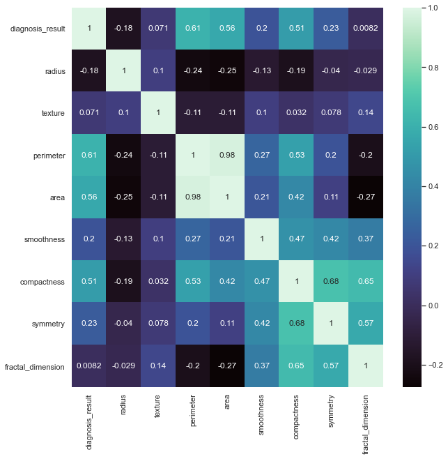
Values = 1 indicate absolute correlation (which makes sense when we compare the same variable to each other). The heatmap legend range tells us where variable correlations approximately lie. Now that we have an idea (quantitatively) of which variables are highly correlated with each other, let's generate some scatter plots to see this visually, too.
# Define the columns and then use the pairplot function in seaborn to plot.

cols = list(df.columns.values)

sns.pairplot(data=df[cols], hue='diagnosis_result', palette='mako')
<seaborn.axisgrid.PairGrid at 0x137418550>
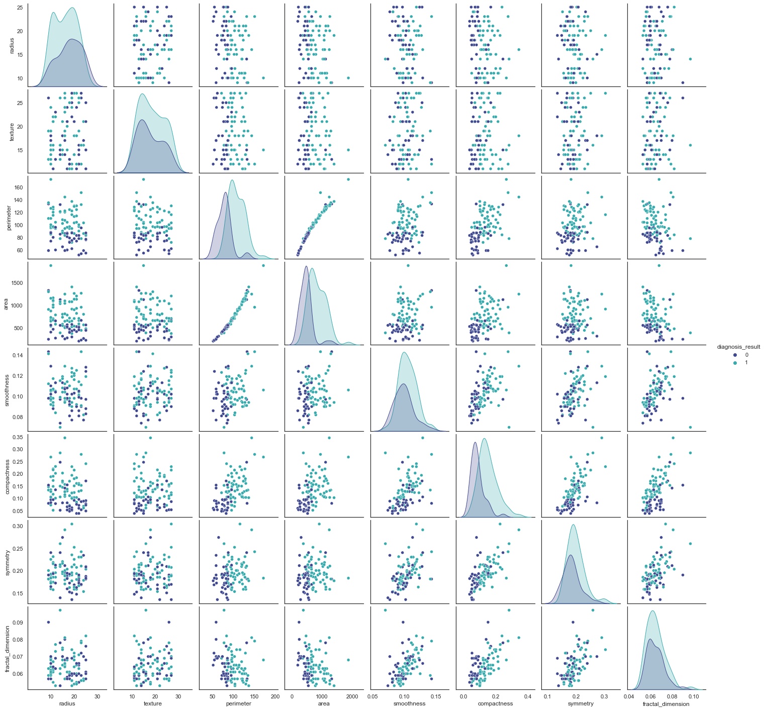
The figures we generated above are very helpful in giving us a visual of what we were seeing with the heatmap quantitatively. We now clearly see that there seems to be a relationship between area and perimeter. This relationship is not quite linear, but almost is. Let’s also create a correlation matrix to confirm this, but so far, there doesn’t seem to be an issue since we don’t have more of these.
# Compute the correlation matrix
corr = df.corr()

# Generate a mask for the upper triangle
mask = np.triu(np.ones_like(corr, dtype=bool))

# Set up the matplotlib figure
f, ax = plt.subplots(figsize=(11, 9))

# Generate a custom diverging colormap
cmap = sns.diverging_palette(230, 20, as_cmap=True)


# Draw the heatmap with the mask and correct aspect ratio
sns.heatmap(corr, mask=mask, cmap=cmap, vmax=.3, center=0,
            square=True, linewidths=.5, cbar_kws={"shrink": .5}, annot=True)

plt.show()
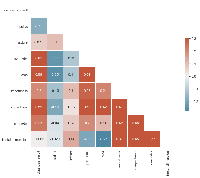
Now, using this correlation matrix, we can confirm that there is not multicolinearity between 2 more predictor variables. In a situation where we saw a variable highly correlated with 2+ predictor variables, we'd have to pick just one of the variables and drop the other columns. This is because otherwise, multicolinearity undermines the statistical significance of an independent variable.
Great! Let's move on to building our machine learning models.
The first thing we will want to do is drop our target ('diagnosis_result') and instead specify this as our dependent variable.
x = df.drop(['diagnosis_result'],axis=1) # drop all columns except the target
y = df['diagnosis_result'] # target is y, aka the result
Now, we will be importing modules from a package called "SciKit-Learn". The reason we didn't just import this module in the very beginnign like the others is because SciKit-Learn is a Python-implemented ML package with tons of frameworks and algorithms. Since we will be using specific ones only today, we can import them as we go along using "from" to give us more control about adding what we need.
First, let's import the module that will allow to split up testing & training data and specify our test size/random state.
from sklearn.model_selection import train_test_split

x_train, x_test, y_train, y_test = train_test_split(x, y, test_size = 0.3, random_state=40)

# Note on the 'random_state' argument: Scikit-learn uses random permutations to generate the splits which ensures that the splits
# that you generate are reproducible.
# Note on test size: generally, it's acceptable to use 70/30 for training/testing data, respectively.
Next we will perform feature scaling. This term refers to making sure all of the values are in the same range (same 'scale') to standardize the data. Otherwise, the ML algorithm will tend to give weight to heigher values and the same vice versa.
from sklearn.preprocessing import StandardScaler

ss = StandardScaler()
x_train = ss.fit_transform(x_train)
x_test = ss.fit_transform(x_test)
Now we will move on to importing the actual ML algorithms that will allow us to make predictions using the data.
We work with Logistic Regression, Decision Trees, Random Forests, KNN, SVM, and the Naïve Bayes Classifier - all core ML frameworks that are widely used in different contexts and applications.
Logisitc Regression
For each algorithm, we will import it from Scitkit Learn, fit the tranining data to the model, and generate predictions.
from sklearn.linear_model import LogisticRegression
lr = LogisticRegression()

# The model takes in the training data, and the prediction takes in the x testing data to generate predictions for y.
model_1 = lr.fit(x_train, y_train)
prediction_1 = model_1.predict(x_test)
Now, we want to compare the training output and testing output. Since the equation to compare the testing accuracy requires the confusion matrix, let's define what a confusion matrix is.
A confusion matrix a table that allows ut to see what the performance of the model is when we use the training data (true values that we know). The following is what a confusion matrix looks like:
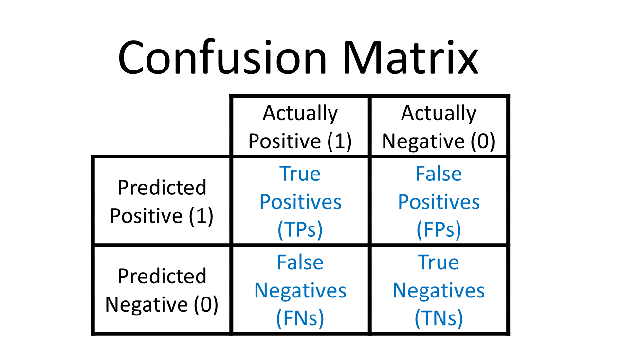
To generate this, we use the command within sklearn.
from sklearn.metrics import confusion_matrix

cm = confusion_matrix(y_test, prediction_1)
print(cm)
[[ 9  1]
 [ 3 17]]
The confusion matrix above tells us the number of times that the model predicts an incorrect output (False Negative, False Negative).
Now we can calculate the testing accuracy.
# Equation for finding Testing Accuracy:

TP = cm[0][0]
TN = cm[1][1]
FN = cm[1][0]
FP = cm[0][1]

print('The Testing Accuracy for Logistic Regression is', (TP+TN)/(TP+TN+FN+FP))
The Testing Accuracy for Logistic Regression is 0.8666666666666667
This means that the Logistic Regression model predicts the correct output 86.7% of the time.
In future models, we can simply use the command within sklearn to do what we just did:
from sklearn.metrics import accuracy_score
accuracy_score(y_test,prediction_1)
0.8666666666666667
We can also generate something called a 'classification report.'
from sklearn.metrics import classification_report
print(classification_report(y_test, prediction_1))
              precision    recall  f1-score   support

           0       0.75      0.90      0.82        10
           1       0.94      0.85      0.89        20

    accuracy                           0.87        30
   macro avg       0.85      0.88      0.86        30
weighted avg       0.88      0.87      0.87        30
Decision Tree Algorithm
# Combine the same steps we did above:

from sklearn.tree import DecisionTreeClassifier
dtc = DecisionTreeClassifier()

model_2 = dtc.fit(x_train, y_train)
prediction_2 = model_2.predict(x_test)
cm2 = confusion_matrix(y_test, prediction_2)
print(cm2)
[[ 9  1]
 [ 5 15]]
accuracy_score(y_test, prediction_2)
0.8
from sklearn.metrics import classification_report
print(classification_report(y_test, prediction_2))
              precision    recall  f1-score   support

           0       0.64      0.90      0.75        10
           1       0.94      0.75      0.83        20

    accuracy                           0.80        30
   macro avg       0.79      0.82      0.79        30
weighted avg       0.84      0.80      0.81        30
Random Forest Algorithm
from sklearn.ensemble import RandomForestClassifier
rfc = RandomForestClassifier()

model_3 = rfc.fit(x_train, y_train)
prediction_3 = model_3.predict(x_test)
cm3 = confusion_matrix(y_test, prediction_3)
print(cm3)
[[ 9  1]
 [ 3 17]]
accuracy_score(y_test, prediction_3)
0.8666666666666667
from sklearn.metrics import classification_report
print(classification_report(y_test, prediction_3))
              precision    recall  f1-score   support

           0       0.75      0.90      0.82        10
           1       0.94      0.85      0.89        20

    accuracy                           0.87        30
   macro avg       0.85      0.88      0.86        30
weighted avg       0.88      0.87      0.87        30
Now we can move onto the next 3 algorithms. >
What's important to remember for the following algorithms is that we need to perform cross validation. Cross validation is a technique used for when the model is prone to overfitting. Overfitting is when the selected too closely mimicks the traning data, and threfore can not make accurate predictions.
Although there are different methods for cross validation, we will employ k-fold cross validation, which is when the data is divided into k subsets. Each time, one of the k subsets is used at the testing data and the rest is left as training data. This is repeated for each of the k subsets, and then the error estimation average of all the k trials is taken to gage how effective the model is. This reduces bias and variance. The reason we used this method over the others is because our dataset is smaller, and removing data would result in underfitting, or when the model is not trained accurately enough to make good predictions.
K-Nearest Neighbor (KNN)
from sklearn.model_selection import KFold
from sklearn.model_selection import cross_val_score
from sklearn.neighbors import KNeighborsClassifier
KNN = KNeighborsClassifier()
kfold = KFold(n_splits = 10)
cv_results = cross_val_score(KNN, x_train, y_train, cv = kfold, scoring = 'accuracy')

model_4 = KNN.fit(x_train, y_train)
prediction_4 = model_4.predict(x_test)
cm4 = confusion_matrix(y_test, prediction_4)
print(cm4)
[[ 6  4]
 [ 2 18]]
accuracy_score(y_test, prediction_4)
0.8
print(cv_results.mean(), cv_results.std())
0.7999999999999999 0.17142857142857143
Support Vector Machine (SVM)
from sklearn.svm import SVC
SVM = SVC()
kfold = KFold(n_splits = 10)
cv_results = cross_val_score(SVM, x_train, y_train, cv = kfold, scoring = 'accuracy')

model_5 = SVM.fit(x_train, y_train)
prediction_5 = model_5.predict(x_test)
cm5 = confusion_matrix(y_test, prediction_5)
print(cm5)
[[ 9  1]
 [ 3 17]]
accuracy_score(y_test, prediction_5)
0.8666666666666667
print(cv_results.mean(), cv_results.std())
0.8285714285714285 0.13997084244475305
Naïve Bayes Classifier
from sklearn.naive_bayes import GaussianNB
NB = GaussianNB()
kfold = KFold(n_splits = 10)
cv_results = cross_val_score(NB, x_train, y_train, cv = kfold, scoring = 'accuracy')

model_6 = NB.fit(x_train, y_train)
prediction_6 = model_6.predict(x_test)
cm6 = confusion_matrix(y_test, prediction_6)
print(cm6)
[[ 9  1]
 [ 6 14]]
accuracy_score(y_test, prediction_6)
0.7666666666666667
print(cv_results.mean(), cv_results.std())
0.7571428571428571 0.20253495541082608
From the 6 different algorithms, the one with the highest accuracy is SVM, Random Forest, and Logisitic Regression -- all of which have an 86.7% testing accuracy. It's important to note that 86.7% is not a very accurate model, especially when it comes to predictions in medicine and patient lives. In these scenarios, it's vital to be as close to 100% as possible. However, in a much larger dataset, the data will usually perform better and tend towards one algorithm with a testing accuract much closer to 100% that we can confidently pick and utilize.
Leave a comment